Analyzing business ownership demographics from Annual Business Survey
Last month, U.S. Census Bureau released its first ever Annual Business Survey ABS, covering statistics of nonfarm employer businesses in 2017. ABS provides business and business owner characteristics such as firms, receipts, payroll and employment by demographic characteristics such as gender, race, ethnicity and veteran status, at regional level.
Today I’m going to demonstrate how to fetch the ABS data using Census API, and explore the demographics of business ownership across cities, counties, and metropolitan areas in the U.S.
Fetch ABS data using Census API
There are many great packages and tutorials that walk you through the process of using Census API, so I won’t go into the details. My favorite one is tidycensus, but unfortunately it’s available for American Community Survey and Decennial Survey only, so I’m going to use censusapi today, which offers a more flexible query structure.
Let’s first take a look at the ABS API endpoints. Navigate to its variables page, it lists all the variables you can query from this API.
Here are the variables I decide to include:
library(tidyverse)
abs_var <- c("GEO_ID", "NAICS2017", "NAICS2017_LABEL", "SEX", "SEX_LABEL", "ETH_GROUP", "ETH_GROUP_LABEL", "RACE_GROUP", "RACE_GROUP_LABEL", "VET_GROUP", "VET_GROUP_LABEL", "FIRMPDEMP", "RCPPDEMP", "EMP", "PAYANN")
Now I’m going to test my query with national data first.
censusapi::getCensus(
  name = "abscs",
  vintage = 2017,
  vars = abs_var,
  region = "us:*",
  key = Sys.getenv("CENSUS_API_KEY")
) %>% head()
## Warning in responseFormat(raw): NAs introduced by coercion
## Warning in responseFormat(raw): NAs introduced by coercion## us GEO_ID NAICS2017 NAICS2017_LABEL SEX SEX_LABEL ETH_GROUP
## 1 1 0100000US 0 NA 003 Male 001
## 2 1 0100000US 0 NA 004 Equally male/female 001
## 3 1 0100000US 0 NA 001 Total 020
## 4 1 0100000US 0 NA 002 Female 020
## 5 1 0100000US 0 NA 003 Male 020
## 6 1 0100000US 0 NA 001 Total 001
## ETH_GROUP_LABEL RACE_GROUP RACE_GROUP_LABEL VET_GROUP VET_GROUP_LABEL
## 1 Total 00 Total 001 Total
## 2 Total 00 Total 001 Total
## 3 Hispanic 00 Total 001 Total
## 4 Hispanic 00 Total 001 Total
## 5 Hispanic 00 Total 001 Total
## 6 Total 00 Total 001 Total
## FIRMPDEMP RCPPDEMP EMP PAYANN
## 1 3480438 10018649629 44854631 1986477555
## 2 859735 1180988058 8030678 272302530
## 3 322076 422573589 2872550 90985526
## 4 78091 74506263 664947 18735668
## 5 206437 309414268 1895189 64179111
## 6 5744643 36579575617 127738274 6534271084Okay, the query returned a data frame, but I noticed that for some reasons NAICS2017 and NAICS2017_LABEL are not displayed properly, and the warning message seems to suggest that this is the result of these two columns being coerced to numerical variables. I spent some time investigating the censusapi::getCensus()’s source code and fixed the bug, which you can see my pull request here.
Let’s run this again with the modified getCensus() function:
getCensus(
  name = "abscs",
  vintage = 2017,
  vars = abs_var,
  region = "us:*",
  key = Sys.getenv("CENSUS_API_KEY")
) %>% head()
## us GEO_ID NAICS2017 NAICS2017_LABEL SEX SEX_LABEL
## 1 1 0100000US 00 Total for all sectors 003 Male
## 2 1 0100000US 00 Total for all sectors 004 Equally male/female
## 3 1 0100000US 00 Total for all sectors 001 Total
## 4 1 0100000US 00 Total for all sectors 002 Female
## 5 1 0100000US 00 Total for all sectors 003 Male
## 6 1 0100000US 00 Total for all sectors 001 Total
## ETH_GROUP ETH_GROUP_LABEL RACE_GROUP RACE_GROUP_LABEL VET_GROUP
## 1 001 Total 00 Total 001
## 2 001 Total 00 Total 001
## 3 020 Hispanic 00 Total 001
## 4 020 Hispanic 00 Total 001
## 5 020 Hispanic 00 Total 001
## 6 001 Total 00 Total 001
## VET_GROUP_LABEL FIRMPDEMP RCPPDEMP EMP PAYANN
## 1 Total 3480438 10018649629 44854631 1986477555
## 2 Total 859735 1180988058 8030678 272302530
## 3 Total 322076 422573589 2872550 90985526
## 4 Total 78091 74506263 664947 18735668
## 5 Total 206437 309414268 1895189 64179111
## 6 Total 5744643 36579575617 127738274 6534271084Looking great! Now the NAICS2017 and NAICS2017_LABEL are displaying correctly.
Now let’s get the data for every metro areas and counties.
cbsa_abs_naics <- getCensus(
  name = "abscs",
  vintage = 2017,
  vars = abs_var,
  region = "metropolitan statistical area/micropolitan statistical area:*",
  key = Sys.getenv("CENSUS_API_KEY")
) %>%
  mutate(GEOID = str_sub(GEO_ID, -5,-1))

stco_abs_naics <- getCensus(
  name = "abscs",
  vintage = 2017,
  vars = abs_var,
  region = "county:*",
  key = Sys.getenv("CENSUS_API_KEY")
) %>%
  mutate(GEOID = str_sub(GEO_ID, -5,-1))
Exploratory Data Analysis
How does business ownership demographics look like in Detroit and Birmingham?
First, let’s specify the GEOIDs of the place of interests. If you are not familiar with census geographies, MCDC has a very friendly GEOID lookup tool.
target_cbsa <- c("19820","13820") # cbsa codes for Detroit-Warren-Dearborn, MI and Birmingham-Hoover, ALNow we can find everything about these two metro areas by filtering the raw data. Use count() to get the codebook of NAICS2017, SEX, RACE_GROUP, ETH_GROUP, VET_GROUP. For example:
cbsa_abs_naics %>%
  count(SEX, SEX_LABEL)
## SEX SEX_LABEL n
## 1 001 Total 119619
## 2 002 Female 15558
## 3 003 Male 18796
## 4 004 Equally male/female 16123
## 5 096 Classifiable 8325
## 6 098 Unclassifiable 7937Let’s take a look at female ownership. So we will get data for female (002), and all businesses that could be classified by gender (096).
cbsa_result <- cbsa_abs_naics %>%
  filter(GEOID %in% target_cbsa) %>%
  filter(SEX %in% c("002","096")) %>%
  filter(NAICS2017 == "72") %>%
  select(GEOID, contains("_LABEL"), FIRMPDEMP, EMP, RCPPDEMP, PAYANN)

cbsa_result
## GEOID NAICS2017_LABEL SEX_LABEL ETH_GROUP_LABEL
## 1 13820 Accommodation and food services Female Total
## 2 13820 Accommodation and food services Classifiable Classifiable
## 3 19820 Accommodation and food services Female Total
## 4 19820 Accommodation and food services Classifiable Classifiable
## RACE_GROUP_LABEL VET_GROUP_LABEL FIRMPDEMP EMP RCPPDEMP PAYANN
## 1 Total Total 256 3404 184036 57926
## 2 Classifiable Classifiable 1479 29483 1736740 482008
## 3 Total Total 1195 20522 1548070 382517
## 4 Classifiable Classifiable 6387 129103 7308642 2047629I’m going to reshape the data to calculate number of firms (FIRMPDEMP), employment (EMP), receipts (RCPPDEMP), and payroll (PAYANN) of female-owed businesses in these two metro areas.
cbsa_result %>%
  pivot_longer(FIRMPDEMP:PAYANN) %>%
  mutate(value = as.numeric(value)) %>%
  select(GEOID, NAICS2017_LABEL, SEX_LABEL, name, value) %>%
  pivot_wider(names_from = "SEX_LABEL", values_from = "value") %>%
  mutate(pct_female = Female/Classifiable) %>%

  ggplot(aes(x = name, y = pct_female, fill = name, label = scales::percent(pct_female, accuracy = 0.1)))+
  geom_col()+
  geom_text(vjust = -0.5)+
  facet_wrap(~GEOID)+
  scale_y_continuous(labels = scales::percent, "share of female owned businesses")+
  theme_classic()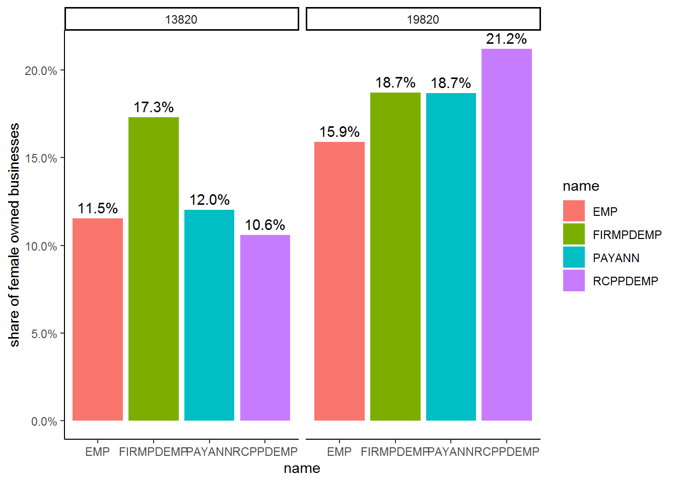
We can see that in the accommodation sector, female business ownership is similar in Birmingham and Detroit (17.3% and 18.7%), but female-owned firms are much smaller in size in Birmingham. They only account for 11.5% of total employment, 12% of payroll, and 10.6% of total sales and receipts.
Scale it up
Let’s write a function to easily adapt this script to explore explore other demographic groups in other regions.
summarise_abs <- function(df, target, col, col_var, NAICS = "00"){
  col <- enquo(col)
  col_LABEL <- paste0((rlang::as_label(col)),"_LABEL")

df %>%
  filter(GEOID %in% target) %>%
  filter(!!col %in% col_var) %>%
  filter(NAICS2017 == NAICS) %>%

  select(GEOID, contains("_LABEL"), FIRMPDEMP, EMP, RCPPDEMP, PAYANN) %>%
  pivot_longer(FIRMPDEMP:PAYANN) %>%
  mutate(value = as.numeric(value)) %>%
  select(GEOID, NAICS2017_LABEL, col_LABEL, name, value) %>%
  pivot_wider(names_from = col_LABEL, values_from = value)
}
Now, let’s look at Asian business ownership in Arlington County, VA (51013)
stco_abs_naics %>%
  summarise_abs("51013",RACE_GROUP, c("60","96"))%>%
  mutate(pct_asian = Asian/Classifiable) %>%
  knitr::kable()
## Note: Using an external vector in selections is ambiguous.
## i Use `all_of(col_LABEL)` instead of `col_LABEL` to silence this message.
## i See <https://tidyselect.r-lib.org/reference/faq-external-vector.html>.
## This message is displayed once per session.| GEOID | NAICS2017_LABEL | name | Asian | Classifiable | pct_asian |
|---|---|---|---|---|---|
| 51013 | Total for all sectors | FIRMPDEMP | 622 | 3655 | 0.1701778 |
| 51013 | Total for all sectors | EMP | 6587 | 50475 | 0.1305002 |
| 51013 | Total for all sectors | RCPPDEMP | 1307860 | 9785745 | 0.1336495 |
| 51013 | Total for all sectors | PAYANN | 384583 | 3182245 | 0.1208527 |
Or, Hispanic business ownership in professional services sector in Austin-Round Rock, TX metro area (12420)
cbsa_abs_naics %>%
  summarise_abs("12420",ETH_GROUP, c("020","096"), "54") %>%
  mutate(pct_hispanic = Hispanic/Classifiable) %>%
knitr::kable()| GEOID | NAICS2017_LABEL | name | Hispanic | Classifiable | pct_hispanic |
|---|---|---|---|---|---|
| 12420 | Professional, scientific, and technical services | FIRMPDEMP | 430 | 8278 | 0.0519449 |
| 12420 | Professional, scientific, and technical services | EMP | 2210 | 51394 | 0.0430011 |
| 12420 | Professional, scientific, and technical services | RCPPDEMP | 289735 | 10400407 | 0.0278580 |
| 12420 | Professional, scientific, and technical services | PAYANN | 123854 | 3865307 | 0.0320425 |